5 Consumer-Resource Dynamics
5.1 The Lotka-Volterra Model
5.1.1 Assumptions
Alfred Lotka (PNAS 1920 6(7):410-415) and Vito Volterra (1926) independently proposed a simple predator-prey model. Lotka was motivated by previous work on rhythmic chemical reactions and oscillations in populations. Volterra was motivated by a question posed by Umberto D’Ancona, a marine biologist who later became Volterra’s son-in-law. D’Ancona was curious if Volterra could use mathematical modelling to explain why the proportion of predatory fish in catches increased when fishing effort decreased during the First World War, and then decreased again when fishing resumed.
The classic Lotka-Volterra model is based on a few simple assumptions.
- Prey grow exponentially at per capita rate \(r\) in absence of the predator.
- Prey are killed at a constant per capita rate \(a\) per predator.
- Each prey killed due to predation gives rise to \(c\) predators.
- Predator death is at a constant per capita rate \(m\).
The model consists of a pair of differential equations. Here \(N\) and \(P\) are the prey and predator densities, respectively.
\[\begin{align}
\frac{dN}{dt} &= rN - aNP, \\
\frac{dP}{dt} &= c aNP - mP.
\end{align}\]
The model has two equilibria:
- the trivial equilibrium \(X_0 = (0,0)\),
- and the interior equilibrium \((\bar{N},\bar{P})\) with
\[\begin{equation*} \bar{N} = \frac{m}{c a}, \qquad \bar{P} =\frac{r}{a}. \end{equation*}\]
5.1.2 Analysis
5.1.2.1 Rescaling
Rescaling is a simple case of dimensional analysis and can be very helpful in analyzing simple models. The basic idea is that we are free to choose the scale of each variable, and with a clever choice of rescalings we can reduce the number of parameters in the model. Let \(N^*\), \(P^*\), and \(t^*\) be arbitrary constants representing the rescalings, and introduce the rescaled variables as \(x = N/N^*\), \(y = P/P^*\), and \(s = t/t^*\). The equations governing the dynamics of the rescaled variables can be found by a simple application of the chain rule to \(N^*x(s) = N(t^*s)\): \[\begin{equation*} N^*\frac{dx}{ds} = \frac{dN}{dt} \frac{dt}{ds} = t^* \frac{dN}{dt} \end{equation*}\] Similarily, \(\frac{dy}{ds} = \frac{t^*}{P^*}\frac{dP}{dt}\). Together, these lead to the equations
\[\begin{align*} \frac{dx}{ds} &= \frac{t^*}{N^*} \left( rN^*x - aN^*xP^*y \strut \right),\\ \frac{dy}{ds} &= \frac{t^*}{P^*} \left( caN^*xP^*y - mP^*y \strut \right). \end{align*}\] The clever trick is to now gather the rescalings and parameters into groups and choose the rescalings to eliminate select groups. \[\begin{align*} \frac{dx}{ds} &= \framebox{$rt^*$}\ x - \framebox{$at^*P^*$}\ xy ,\\ \frac{dy}{ds} &= \framebox{$cat^*N^*$}\ xy - \framebox{$mt^*$}\ y . \end{align*}\] This leaves us with four groupings and three rescalings to choose. In general, we would expect to be able to choose the rescalings to set three of the groups to one. Another option is to choose the scalings to set two groups equal to one another. For example, we can choose the rescalings to satisfy the three conditions \[\begin{gather*} rt^* = 1, \\ at^*P^*=1, \\ cat^*N^*=mt^*. \end{gather*}\] Solving these leads to the rescalings \(t^* = 1/r\), \(N^* = m/(ca)\) and \(P^* = r/a\). Introducing the new rescaled parameter \(\mu = m/r\), we find
\[\begin{aligned} \frac{dx}{dt} &= f(x,y) = x(1 - y), \\ \frac{dy}{dt} &= g(x,y) = \mu y(x - 1), \end{aligned} \tag{5.1}\]
Our interpretation of the scalings is that time is measured relative to the growth rate of the Prey, Prey densities are measured relative to the ratio of the prey mortality and the prey growth rate per predator, which we previously found to be the equilibrium prey population, and prey densities are measured relative to the ratio of the prey growth rate and the attack rate, which we found to be the equilibrium predator population. The resulting single parameter \(\mu\) is a rescaled predator mortality (\(\mu = m/r\)).
5.1.2.2 Phase Plane Analysis
We refer to the set of points \((x,y)\) with \(x\ge0\) and \(y\ge0\) as our state space. Geometrically, Equations Equation 5.1 specify a vector field on the state space, and solutions of the equations are curves which are tangent to these vectors at each point. A point \((x,y)\) for which \(f(x,y)=g(x,y)=0\) is an equilibrium solution: these are constant solutions satisfying the differential equations.
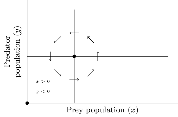
Solutions to \(f(x,y)=0\) and \(g(x,y)=0\) are referred to as the \(x\)-nullclines and \(y\)-nullclines respectively. For the Lotka-Volterra model, the \(x\)-nullclines are the lines \(x=0\) and \(y=1\), and the \(y\)-nullclines are the lines \(y=0\) and \(x=1\). The nullclines intersect at the equilibria. The prey population is decreasing on one side of the prey-nullcline, increasing on the other, and the solutions cross the prey-nullcline parallel to the predator-axis. Hence, the nullclines partition the state spatce into regions where populations are increasing or decreasing. Since the nullclines of the Lotka-Volterra model are vertical and horizontal lines, a simple check of the signs of \(f\) and \(g\) in each of the four regions shows that solutions must oscillate counterclockwise around the nontrivial equilibrium.

Another trick that often provides insight is to consider the solutions curves as graphs of a function \(y(x)\). Since, under reasonable conditions, \(\dfrac{dy}{dx} = \dfrac{dy}{dt}/\dfrac{dx}{dt}\), combining the two equations leads to a differential equation for \(y(x)\). \[\frac{dy}{dx} = \frac{\mu y(x - 1)}{x(1 - y)}. \tag{5.2}\] This can be integrated as \[\Psi(x,y) = \mu (x - \log x) + y - \log y. \tag{5.3}\]
Solutions of Equation 5.2 are level curves of \(\Psi\). Since \(\Psi\) is concave in the positive quadrant, these will be closed curves, or periodic orbits, surrounding the interior equilibrium.
Now let \(T\) be the period of oscillation of a particular solution to the model. From Equation 5.1 we have \[\begin{align*} \frac{1}{T}\int_{x(t_0)}^{x(t_0+T)} \frac{1}{x}\, dx = 1-\frac{1}{T}\int_{t_0}^{t_0+T} y(t)\, dt, \\ \text{and}\quad \frac{1}{\mu T}\int_{y(t_0)}^{y(t_0+T)} \frac{1}{y}\, dy = \frac{1}{T}\int_{t_0}^{t_0+T} x(t)\, dt - 1. \end{align*}\] Since the solutions are periodic with period \(T\), the integrals on the left are zero. The integrals on the right are simply the mean values of \(x\) and \(y\) over one full period. Hence, we conclude that the mean populations on any orbit are equal to the equilibrium populations. Volterra concluded from this that an intervention in a predator-prey system that removes both predator and prey with equal effort, will result in increased average prey populations.
5.2 Generalized Lotka-Volterra Models
5.2.1 The Volterra Model
In 1931, Volterra published an analysis of a predator-prey model with a prey carrying capacity: \[\begin{align} \frac{dN}{dt} &= rN\left(1-\frac{N}{K}\right) - aNP, \\ \frac{dP}{dt} &= c aNP - mP. \end{align}\] The model can be rescaled to yield \[\begin{align} x' &= x\left(1-\frac{x}{\kappa}\right) - xy, \\ y' &= \mu y(x - 1). \end{align}\]
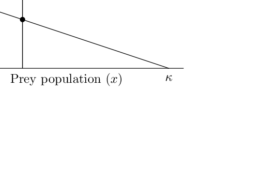
These equations represent a similar vector field to the original Lotka-Volterra model. The \(x\) nullcline is no longer horizontal, but has the equation \(y= 1- x/\kappa\). The interior equilibrium is at \(x=1\), \(y=1-1/\kappa\), which is positive only if \(\kappa > 1\).

Computations show the interior equilibrium to be stable, the trivial equilibrium to be a saddle, and the solutions are oscillations decaying to the interior equilibrium.
5.2.2 The Rosenzweig-MacArthur Model
Rosenweig and MacArthur (1963) are credited with the addition of a hyperbolic functional response to the classic predator-prey model. \[\begin{aligned} \frac{dN}{dt} &= rN\left(1-\frac{N}{K}\right) - \frac{aNP}{1 + bN}, \\ \frac{dP}{dt} &= c \frac{aNP}{1 + bN} - mP. \end{aligned} \tag{5.4}\]
They assume that the rate predators kill prey increases linearly with prey at small densities, but saturates at higher prey densities. The numerical response is taken to be proportional to the functional response, just as in the simpler Lotka-Volterra model.
The model has a trivial equilibrium at \((0,0)\) and a predator-free equilibrium at \((0,K)\). There is a single interior equilibrium \((\bar{N},\bar{P})\) with \[\begin{align*} \bar{N} &= \frac{m}{ca-mb}, \\ \bar{P} &= r\bar{N}(1+b\bar{N})\left(1-\frac{\bar{N}}{K}\right). \end{align*}\] For both \(\bar{N}\) and \(\bar{P}\) to be positive, we must have \(0 < \frac{m}{ca-mb} < K\)
A stability analysis of the interior fixed point is simplified by writing the system in the Kolmogorov form \[\begin{aligned} \frac{dN}{dt} &= Nf(N), \\ \frac{dP}{dt} &= Pg(P), \end{aligned} \tag{5.5}\] where \[f(N,P) = r\left(1-\frac{N}{K}\right) - \frac{aP}{1 + bN},\qquad g(N,P) = c \frac{aN}{1 + bN} - m.\] The interior equilibrium satisfies \(f(\bar{N}) = g(\bar{P}) = 0\).
The Jacobian at \((\bar{N},\bar{P})\) is \[\begin{equation*} \begin{pmatrix} \bar{N}\bar{f}_N & \bar{N}\bar{f}_P \\ \bar{P}\bar{g}_N & \bar{P}\bar{g}_P \end{pmatrix} \end{equation*}\] where a bar over a function indicates evaluation at the interior equilibrium. Note that \(\bar{g}_P = 0\), \(\bar{f}_P < 0\) and \(\bar{g}_N>0\), so that the determinant of \(J\) is always positive, and the trace of \(J\) is \[\text{tr}(J) = \bar{N}\bar{f}_N = \frac{rbca}{ca-bm}\left( \frac{ca - bm}{ca} - \frac{1}{Kb}\right).\] Hence, according to the Hopf Birfurcation Theorem, the equilibrium changes from a stable to unstable focus as \(\bar{f}_N\) changes from positive to negative. It can further be shown that a stable limit cycle bifurcates from the equilibrium as the trace increases through zero.
The equilibrium destabilizes as \(Kb\) is increased or as \(\frac{bm}{ca}\) is decreased. The former is often referred to as the paradox of enrichment. The simple Rosenzweig-MacArthur model predicts that an increase in the \(K\), the carrying capacity of the prey, can destabilize the equilibrium.
5.3 The Functional Response
Turchin (2003) provides an excellent discussion of the various responses of predators to changes in prey populations. Consider a general predation model of the form
\[\begin{aligned} \frac{dN}{dt} &= NF(N) - H(N,P)P, \\ \frac{dP}{dt} &= G(N,P)P - mP. \end{aligned} \tag{5.6}\]
The three functions are usually referred to as - the net per capita growth rate \(F\), which is assumed independent of predation, - the functional response \(H\), which is the rate individual predators kill prey, and - the numerical response \(G\), which models the dependence of the per capita predator growth rate on population densities.
Holling (1959) introduced a simple classification of functional responses of predators into type I, II, or III (see Figure 5.3). Mathematically, type I and II are similar, and represent a saturating response.

5.3.1 Phase Planes and Linear Stability Analysis
Consider the pair of differential equations \[\begin{aligned} \frac{dx}{dt} &= f(x,y), \\ \frac{dy}{dt} &= g(x,y), \end{aligned} \tag{5.7}\] with initial conditions \(x(0) = x_0\), \(y_0=y_0\). A system of differential equations that does not depend explicity on the independent variable is said to be autonomous. Since we are usually interested in nonnegative solutions to these equations, the state-space of interest is the set \((x,y)\) with \(x\ge0\) and \(y\ge 0\). A solution to the differential equations consists of a pair of functions, \(x(t)\) and \(y(t)\), which, with reasonable restrictions on \(f\) and \(g\), will be continuous and differentiable if not for all \(t\ge0\) then at least for some interval \([0,T)\). Thus, solutions are either points or curves in the state space, parameterized by the independent variable, \(t\). An equilibrium solution of Equation 5.7 is a constant solution \((x(t),y(t)\) satisfying \(f(x(t),y(t)) = g(x(t),y(t)) = 0\). This can be visualized as a point in state-space.
Geometrically, Equation 5.7 specifies a vector field on the state space. A solution passing through some point \((x,y)\) at time \(t\) can be viewed as a curve tangent to the vector \((f(x,y),g(x,y))\).
Solutions to \(f(x,y)=0\) and \(g(x,y)=0\) are referred to as the \(x\)-nullclines and \(y\)-nullclines respectively. The equilibrium solutions are found at the intersections of these nullclines. The nullclines partition the state spatce into regions where the \(x\) and \(y\) components of the solutions are increasing or decreasing.
In our analysis of the scaler differential equation, \(\dot{x}=f(x)\), we found that the stability of an equilibrium solution, \(x^*\), was determined by the slope \(f'(x^*)\). If \(f'(x^*)>0\), then \(x(t)\) must be decreasing if \(x(t)<x^*\) and increasing if \(x(t)>x^*\). Thus solutions near \(x^*\) move away from \(x^*\) if \(f'(x^*)>0\), but move towards \(x^*\) if \(f'(x^*)<0\).
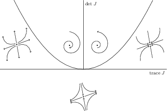
Let \(J\) denote the matrix of partial derivatives of \(f\) and \(g\) evaluated at the equilibrium: \[\begin{equation} J = \begin{pmatrix} f_x(x^*,y^*) & f_y(x^*,y^*) \\ g_x(x^*,y^*) & g_y(x^*,y^*) \end{pmatrix} \end{equation}\] Near the equilibrium, we can expand the right hand side of the model as a Taylor series about \((x^*,y^*)\): \[\begin{equation} \begin{pmatrix} \frac{dx}{dt} \\ \frac{dy}{dt} \end{pmatrix} = \begin{pmatrix} f(x^*,y^*) \\ g(x^*,y^*) \end{pmatrix} + J \begin{pmatrix} (x-x^*) \\ (y-y^*) \end{pmatrix} + \dots \end{equation}\] Since \(f\) and \(g\) are zero at an equilibrium, the linearized system is determined by the matrix \(J\). There is an important theorem that states that the dynamics of the nonlinear system are topologically equivalent to the dynamics of the linearized system provided all the eigenvalues of \(J\) have nonzero real part. The stability of the equilibrium and qualitative nature of the solutions near the equilibrium can be determined from the eigenvalues of \(J\) provided none of the eigenvalues of \(J\) have zero real part.
Let \(u = \begin{pmatrix} (x-x^*) \\ (y-y^*) \end{pmatrix}\). Then the linearized system is simply \(\dot{u} = Ju\). Now suppose \(v\) is an real eigenvector of \(J\) associated with the real eigenvalue \(\lambda\). Since, \(Jv = \lambda v\), we can find a solution in the direction of lambda by setting \(u(t) = a(t)v\) for a scalar function \(a\). \[\dot{a}v = Jav = \lambda av \Rightarrow \dot{a} = \lambda a \Rightarrow a(t) = a(0)e^{\lambda t}\] With a few more theorems on the uniqueness of solutions and linear combinations of solutions that can be found in Logan (2006) we can distill the results down to the diagram of Figure 5.4.
