Show the code
plot(NULL,xlim=c(-2,2),ylim=c(-2,2),xlab = "x(t)", ylab = "y(t)")
abline(0,1/2,col='red')
abline(0,-3/2,col='green')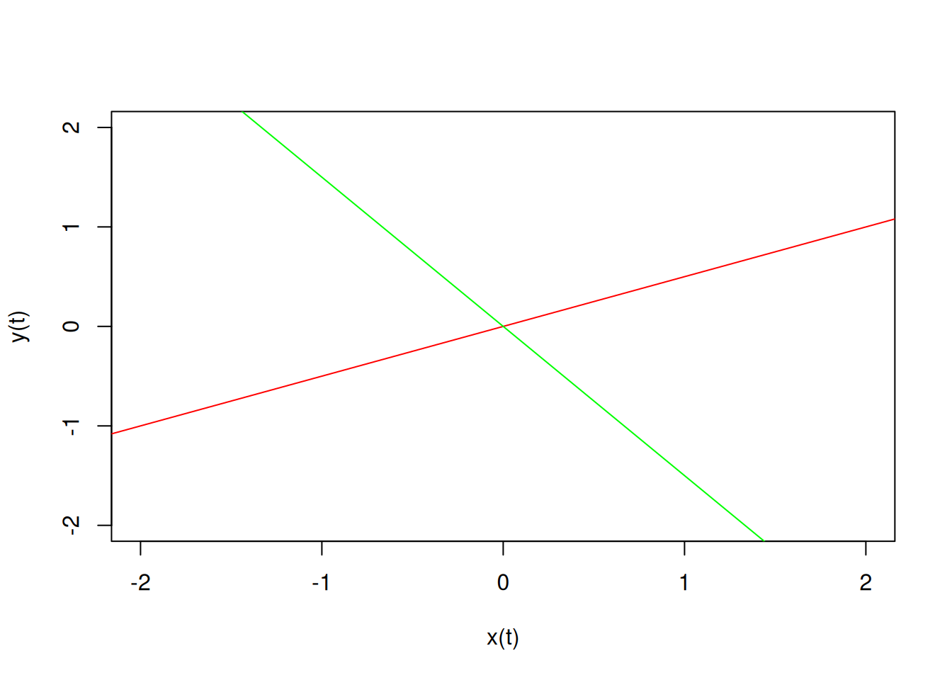
Show the code
p = recordPlot()Consider differential equations of the form \(\dot{x} = Ax\) where \(A\) is an \(n\times n\) matrix of real numbers. For convenience, we’ll use \({\mathbb R}^{n\times n}\) to denote the set of all such matrices.
Integrating the equation we have \(x(t) = x_0 + \int_0^t Ax(s)\, dx\), which we can view as a map on the set \({\mathbf C}^1(0,t)\) of differentiable functions on \((0,t)\). If we iterate this map starting with the constant function \(x_0\), we find \[\begin{aligned} x_1 &= x_0 + Ax_0t \\ x_2 &= x_0 + Ax_0t + \frac{1}{2}A^2x_0t^2 \\ x_3 &= x_0 + Ax_0t + \frac{1}{2}A^2x_0t^2 + \frac{1}{6}A^2x_0t^3 \end{aligned}\]
If \(A\) is a scalar, or a \(1\times 1\) matrix, this iteration generates the familiar series for the exponential. In particular, \(x_n\) converges to \(e^{At}x_0\).
We’ll anticipate that the series also converges in a meaningful way if \(A\) is a matrix, and denote the limit by the matrix exponential, \(e^{At}\).
Exercise 7.1 Show that \(x_n\) converges if \(A\) is an \(n\times n\) matrix. See the section on the matrix exponential in Hirsch, Smale, and Devaney (2013) for a hint.
Example 7.1 Construct a phase portrait for the system \[\begin{aligned} \dot{x} &= 3x + 4y \\ \dot{y} &= 3x - y \end{aligned}\]
The eigenvalues are 5 and -3, and the corresponding eigenspaces are the spans of \(\begin{pmatrix} 2 \\ 1 \end{pmatrix}\) and \(\begin{pmatrix} 2 \\ -3 \end{pmatrix}\) respectively.
The solutions corresponding to these eigenvalue/eigenvector pairs trace out the eigenspaces in the \(x\)-\(y\) plane.
plot(NULL,xlim=c(-2,2),ylim=c(-2,2),xlab = "x(t)", ylab = "y(t)")
abline(0,1/2,col='red')
abline(0,-3/2,col='green')
p = recordPlot()The general solutions to the system are linear combinations of the two solutions corresponding to the eigenvalues. Since the eigenvalues have opposite signs, these trace out hyperbolae. To see this, let \(a(t)\begin{pmatrix} 2 \\ 1 \end{pmatrix} + b(t) \begin{pmatrix} 2 \\ -3 \end{pmatrix}\) with \(a(t) = a_0e^{5t}\) and \(b(t) = b_0e^{-3t}\) denote the general solution. This is a curve, parameterized by \(t\) for \(-\infty < t < \infty\). The coefficients, \(a(t)\) and \(b(t)\) satisfy \(a^3b^5 = a_0^3b_0^5\). These are hyperbolae in the \(a\)-\(b\)-plane which are hyperbolae in the \(x\)-\(y\) plane asymptotic to the two eigenspaces.
a_0 = 1/5
b_0 = 1/5
a = a_0*2**seq(-5,5,length=21)
b = b_0/(a/a_0)**(3/5)
x = 2*a+2*b
y = a - 3*b
replayPlot(p)
lines(x,y,col='blue')
lines(-x,-y,col='blue')
x = -2*a+2*b
y = -a - 3*b
lines(x,y,col='blue')
lines(-x,-y,col='blue')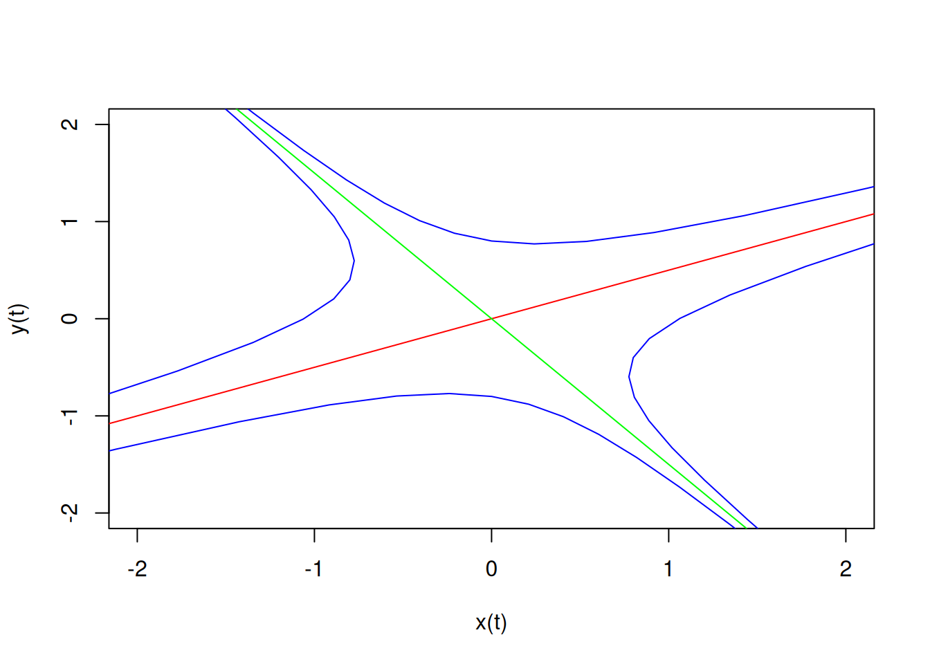
# abline(0,-3/4)
# abline(0,3)
# x = seq(-2,2,length=20)   # be sure to skip over zero (why?)
# segments(x,-3*x/4-.05,x,-3*x/4+.05)
# segments(x-.05,3*x,x+.05,3*x)
```
There are two sets of subspaces (i.e., two pairs of lines) that we can use to construct the diagram.
The \(x\) and \(y\) nullclines of the systems are the sets where \(\dot{x}=0\) and \(\dot{y}=0\), respectively. For this example, those are the lines \(3x+4y=0\) and \(3x-y=0\). Solutions cross these lines vertically (\(\dot{x} = 0\)) and horizontally (\(\dot{y}=0\)), respectively.
Example 7.2
Example 7.3